Linear regression very simply explained

Susan Brommer | 14 November 2021 | data science, models

What is linear regression?

Linear regression is perhaps the most basic example of modern statistical modeling and data science. Regression is a method that attempts to determine the relation between some variables. For example, the salary of a worker depends on how many hours they worked. There is a relation between the worker’s hours and their salary. Regression tries to grasp this relation.

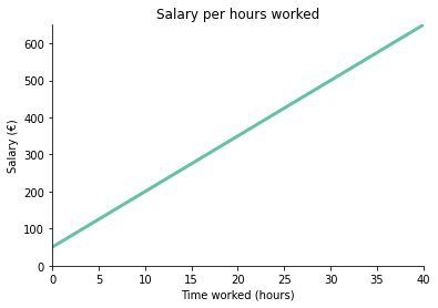
The linearity in linear regression tells us we are looking for a linear relation. Such a relation would look like the figure below. We see on the x-axis the hours a worker worked, and on the y-axis their salary. When the hours increase, the salary increases as well. It’s a nice straight line, and that tells us the relation is linear. With regression we can look for al kinds of different lines. But with linear regression specifically, we look for a straight relation like this.

So what?

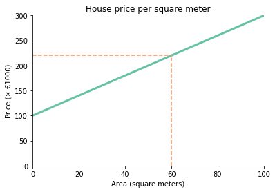
Linear regression is actually pretty useful. Why? Because we can predict the future! Say we want to buy a house, but we do not know how much the seller is going to ask. If we do know the floor area of the house, and the relation between floor area and house prices, we can predict what the price will be. Say that the house we’re interested in has a floor area of 60 square meters. If we look at the figure below, we can see that the price is probably going to be around €220.000.

The math

Let’s look at the math behind a linear relationship. In the examples we have seen already, there are always two variables. One of those variables depends on the other. In case of the worker’s salary, the variables are the hours worked and the salary. The salary depends on the hours worked. We call the salary the dependent variable, and the hours worked the independent variable. Looking at the figure, we see that if the worker does not work any hours, his salary is approximately €50. And then for every hour worked, his salary goes up by about €15. We can express this in a formula:

salary = 50 + 15 × hours

We can do something similar for the housing prices. The variables are the floor area and the house price. The house price depends on the floor area. We call the price the dependent variable, and the area the independent variable. The figure tells us that the base price for a house is €100.000. For every square meter, the price increases by €2.000. Mathematically, we formulate it like this:

price = 100,000 + 2,000 × area

When we want to predict the price for a house with an area of 60 square meters, we simply plug in 60 into the the formula, and calculate the outcome:

price = 100,000 + 2,000 × 60 = 220,000

Mathematicians love to generalise formulas. We can already see a pattern in the two examples above. The general formula for a linear relation is:

Y = b + m × X

• Y is the dependent variable, or the value that we want to predict,
• X is the independent variable, or the value that we have knowledge about,
• m is called the slope, and tells us how much Y increases for every increase in X
• b is called the intercept, and gives us the base value for Y, or the value of Y if X is zero.

Regression in action

We now know what a linear relation is, and we even know how to formulate it in mathematics. The problem is that not every relation in the world is a perfect linear relation. Your salary might directly depend on the hours you work. But no house price depends on floor area alone. There are lots of other factors, like number of rooms, the neighbourhood, and distance to the nearest highway. And even if we knew all other factors, there would still be some noise and randomness.

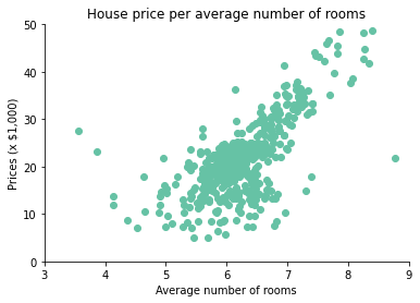
Lets look at some actual housing data. The data we look at comes from the Boston Standard Metropolitan Statistical Area in 1970. Every point that we see represents a Boston suburb. On the x-axis we see the average number of rooms of houses. On the y-axis we see the average housing price. Even though the points do not perfectly lie on a straight line, we can very well imagine a line going from the bottom left to the upper right that follows the points as best as it can.

And that is exactly what linear regression does. It looks at all these points, and finds the best fitting line. Not all points will lie on this line. That is simply impossible. Every point will have a distance to this line. If you sum up the distance of every point to the line, then you get the total distance. And linear regression finds the line with the smallest total distance.

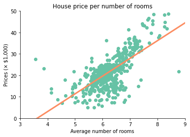
Let’s see linear regression in action. Remember the linear formula Y = b + m × X? We can give the regression model the data that we have, and then ask for the values for b and m. It returns for the intercept b the value -30. The slope m is approximately 8.27. This gives us the formula:

price = -30,000 + 8,270 × rooms

Linear regression has just given us the linear relation between the number of rooms and the housing price. We can draw this linear relation on top of the data points. The result seems pretty good. The line follows the data points as good as it can. We can now use this line to predict housing prices in Boston (at least, in 1970). If we know the number of rooms in a house, we can give an estimate of its price.

You want more?

Hopefully this article gave you a little bit of insight into one of the most basic modeling techniques. If you are interested in a little bit more math about how linear regression actually finds this line, look at my article about the mathematics of linear regression which I will publish soon. If you are interested in some more advanced linear regression, read my article about the Boston housing data set, which I will also publish soon.